Plotting Lissajous Curves with Parametric Equations.
We only need the position equations to plot the Lissajous Curve.
These are simple parametric curves.
This topic here is only because they look nice to me!
Parameters Equations
Add parametric equations in the Math FB to calculate the X,Y coordinates of a Lissajous Curve.
The parametric equations for the Lissajous Curve of curves are:
x = cos(a*t)
y = sin(b*t)
If you change a parametric-constants (a or b), you will plot a different Lissajous Curve.
Parameters and Variables
a = the frequency of the motion along the X-axis
b = the frequency of the motion along the Y-axis
t = the independent variable: 0 to 360 (or 2*pi)
Three(3) Inputs: a, b, and t
Two(2) Outputs: x and y.
|
|
Input-Connector and Output-Connectors
|
Input-Connectors
We need three input-connectors: three parameters (a, b) and one variable (t)
1.Double-click the Math FB to open a Math FB dialog
2.Click the Add Input button three time to add three input-connectors to the Math FB
3.Click the Update button |
|
|
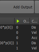
Output-Connectors
We need two output-connectors for the X-axis and Y-axis motion-data
1.Double-click the Math FB to open the Math FB dialog
2.Click the Add Output button to add two outputs from the Math FB
The unit of the output data is dependent on the Output Data Type.
3.Set the Output Data Type to Linear Coordinates
4.Click the Update button |
|
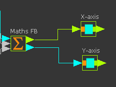
Parametric Equations in the Math FB
Equations for the Position (Displacement) for the two outputs.
The Lissajous equations for the X and Y coordinates are given here again:
•x = cos(a×t) ..... Equation 1
•y = sin(b×t) ..... Equation 2
We must re-write these for the Math FB.
|
|
 Lissajous equations - position only |
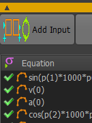
The Equations in the Math FB
We use
p(0) as t
p(1) as a
p(2) as b
1.Enter the equations carefully - see the image to the left.
•Equation 1 = cos((p(1)× 1000)× p(0))
•Equation 2 = sin((p(2)× 1000)× p(0))
2.Click Update button to confirm changes. |
What about the Units and Range of the Equations
The Sin and a Cos functions produce a a minimum value of -1 and a maximum of 1. (±1)
Inside the Math FB, all parameters are SI units. A range of ±1 is a range of ±1 meter (1)
Outside the Math FB, a range of ±1 is a range of ±1000.
Typically, you scale the motion to reduce its range.
To scale the motions:
•Use Gearing FBs: e.g. if you use a Gearing Ratio = 0.1, there is a motion range of ±100 at the X-axis and Y-axis Sliders
or
•Edit the equations in the Math FB. e.g. if you divide each equation by 10, there is a motion range of ±100 at the X-axis and Y-axis Sliders
<<<< see the image: each equation now has a range of ±100
|
|
 Reduce the motion range
by a factor of 10 |
The Piggyback Slider Model for the Lissajous Figures
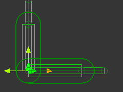
|
The Mechanical model in MechDesigner
|
|
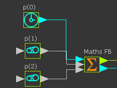
The Math FB - input connectors
•t .... the angle of the function from 0 to 2*pi - the output from a Linear-Motion FB
•a ... the frequency of oscillation of the X-axis - add and edit the Gearing FB > Add after Gearing-Ratio parameter.
•b ... the frequency of oscillation of the Y-axis - add and edit the Gearing FB >Add after Gearing-Ratio parameter.
Note:
Outside the Math FB, a range of t is 0 - 360 degrees
Inside the Math FB, a range of t is 0 - 20*pi radians
|
|
|
Math FB - output variable connectors
The Math FB has two output-connectors
•x ... the horizontal position of the X-Slider
•y ... the vertical position of Slider-Y |
|
 Video of Lissajous Curves - Click to Play |
The Trace-Point of the Piggyback Slider
Add a Trace-Point to show the Path of a Point moving with the Y-axis Slider.
Edit the Gearing FB values to
|
|
