Point-Data FB and Measurement Function-Blocks
The Point-Data FB and the Measurement FB have output-connectors, and do not have input-connectors..
Use a:
•Point-Data FB to measure the position and motion of a Point*, relative to the origin of the Base-Part.
•Measurement FB to measure the motion of one sketch-element relative to another - usually in different Parts.
The motion-values at the output-connectors of these FBs provide the measurements AND also their first and second motion-derivatives.
* In all cases below, we use the term Point to mean Point, start-Point, end-Point, center-Point, and Motion-Point.
Motion-Dependency
Motion-Dependency is the term we use when the motion of a kinematic-chain is a function of the motion of a different kinematic-chain.
In two examples below (5.7-B and 5.7-C) there are TWO kinematic-chains.
•Kinematic-chain A : here a Crank. We connect a wire from a Linear-Motion FB to the input of a Motion-Dimension FB.
We measure, with Measurement FB (A), the distance from a stationary Point in the Base-Part to the end-Point of the Crank. The distance continually changes as we cycle the model.
The output from the Measurement FB (A) provides not only the distance between the two Points, but also the first and second motion-derivatives of the distance between the two Points.
•Kinematic-chain B: here a Slider. It takes the motion-values at the output from the Measurement FB (A) as the motion and input to the Motion-Dimension FB, for the Slider.
We will use a Graph FB to plot the motion-values measured by a Point-Data FB. |
|
|
Use a Point-Data FB to make a plot of the position and motion of a Point* relative to the Origin of the Base-Part. |
STEP 1: Assemble a kinematically-defined chain. Add a Crank - see image below. Edit the Base-Value of the Motion-Dimension FB to 0. Use the Part-Editor to edit the Crank. Edit its length to be 50mm. Use the Part-Editor to edit the Base-Part. Edit the length of the Line to be 60mm STEP 2: Click Kinematics FB toolbar > Add Point-Data FB STEP 3: Click the graphics-area The Point-Data FB is now in the graphics-area. Link the Point-Data FB with a Point*. STEP 4: Double-click the Point-Data FB - the Point-Data dialog is now open. We need to select a moving Point* in a Part that is kinematically-defined. STEP 5: Click the end-Point of the Crank STEP 6: Click Now the end-Point of the Crank is linked to the Point-Data FB. Add a Graph FB: STEP 7: Click Kinematics toolbar > Add Graph FB STEP 8: Click the graphics-area The Graph FB is now in the graphics-area. Connect wires from the Point-Data FB to the Graph FB: STEP 9: Drag to connect a wire from the top and middle output-connector of the Point-Data FB to input-connectors of the Graph FB STEP 10: Connect a Linear-Motion FB to the X-axis of the Graph FB (the bottom connector) - although not required. STEP 11: Double-click the Graph FB in the graphics-area. The Plot / Graph is now open. |
|
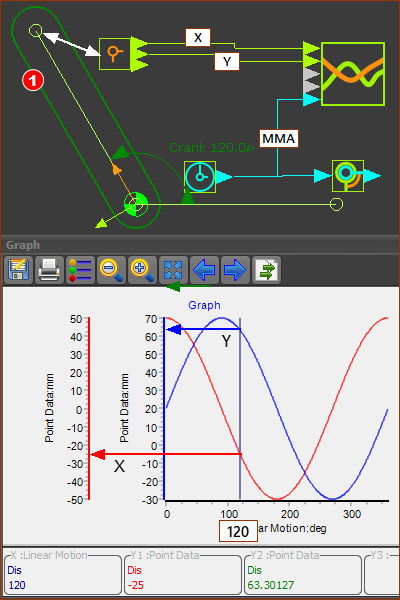
After you follow these steps, you can see all of the elements in the image below. The X-axis of the Graph is equal to the MMA. |
|
|
|
In this model, the Pin-Joint for the Part is 20mm above the 0,0 of the Base-Part and Mechanism-Editor. The horizontal and vertical motions at the end-Point of the Crank are sinusoidal, with an amplitude 50mm. The sinusoid for Y lags the X value by 90º. The MMA angle is set to 120º, as shown by the vertical line/cursor in the Graph. The DROs (Digital Readouts), below the Graph, give the Y1 (=X coordinates of the Point), and Y2 (=Y coordinates of the Point). You can see: •the Blue graph has a range of -30 to +70mm •the Red graph has a range -50 to +50mm |
|
Top-Tip To show the position, velocity and acceleration of a Point in the same graph. 1.Drag a wire from the same output-connector of the Point-Data FB three times to three different input-connectors on a Graph FB. 2.Use the Y-axis display options in the Graph dialog to display each motion derivative. |
|
|
Use a Measurement FB to get the motion-values from Kinematic-Chain A for Kinematic-Chain B |
STEP 1: Assemble Kinematic-Chain A We will use the Crank in the model above - 5.7-A STEP 2: Assemble a Kinematic-Chain B To keep it simple, a Slider STEP 3: Double-Click the Motion-Dimension FB for the Slider to open the Motion-Dimension dialog STEP 4: Edit the Base-Value parameter to 0. STEP 5: Close the dialog. Add a Measurement FB STEP 6: Click Kinematics toolbar > Add Measurement FB STEP 7: Click a Point in the Base-Part and then the end-Point of the Crank STEP 8: Click the graphics-area The Measurement FB (and dimension) are now in the graphics-area. Connect the Kinematic-Chains. STEP 8: Connect a wire from the TOP output-connector of the Measurement FB to the Motion-Dimension FB that controls the motion and position of the Slider. Now, Kinematic-Chain B has Motion-Dependency on Kinematic-Chain A Add a Graph FB: STEP 9: Click Kinematics toolbar > Add Graph FB STEP 10: Click the graphics-area The Graph FB is now in the graphics-area. Connect wires to the Graph FB: STEP 11: Connect a wire from the output of the Motion-Dimension FB of the Slider to the input of the Graph FB STEP 12: Connect a Linear-Motion FB to the X-axis of the Graph FB (the bottom connector) STEP 13: Double-click the Graph FB in the graphics-area The Plot / Graph is now open. |
|
|
|
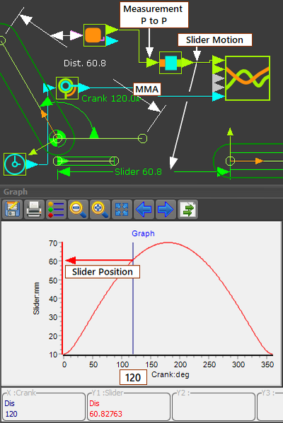
The Measurement FB includes the distance between two Points. The distance between the two Points continually changes as the 'machine' cycles. The Base-Value parameter in the Motion-Dimension dialog for the Slider and the Crank are zero(0). Therefore, the position of the Slider is equal to the distance as defined by the Measurement FB and the output from its Motion-Dimension FB The distance between two Points is 60.8mm. Therefore, in this case, the position of the Slider is also 60.8mm |
|
+
|
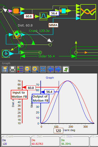
We will use the model above. Also add a Motion FB. Kinematic-Chain B uses the output from a Measurement FB of Kinematic-Chain A as the input to a Motion FB. The output from the Motion FB is the input to the Slider , which is Kinematic-Chain B |
STEP 1: Assemble Kinematic-Chain A and Kinematic-Chain B We will use the Crank and Slider in the model above - 5.7-B - but edit the lengths of the Crank and the Line in the Base-Part. Edit the length of the Crank to be 40mm, and the length of the Line in the Base-Part to be 30mm STEP 2: Delete the wire from the Measurement FB to the Motion-Dimension FB for the Slider STEP 3: Add a Motion FB to the graphics-area STEP 4: Connect a wire from the TOP output-connector of the Measurement FB to the input of the Motion FB. STEP 5: Connect a wire from the Motion FB to the Motion-Dimension FB for the Slider. Now the Kinematic-Chain B is dependent on Kinematic-Chain A. Now connect wires to a Graph FB: STEP 6: Connect a wire from the TOP output of the Measurement FB to Y-2 input on the Graph FB STEP 7: Connect a wire from the output of the Motion-Dimension FB for the Slider to Y-1 input of the Graph FB STEP 8: Connect a wire from the Linear-Motion FB to the X-axis of the Graph GB STEP 9: Double-click the Graph FB in the graphics-area. AND, connect wires to a Graph FB STEP 10: Connect a wire from the output of the Motion-Dimension FB for the Slider to a Y-axis input of the Graph FB STEP 11: Connect a wire from the TOP output of the Measurement FB to a X-axis input on the Graph FB STEP 12: Double-click the Graph FB in the graphics-area. |
|
The input to the Motion FB is from the output from the Measurement FB: •may be greater than 360 •may be quite complex Irrespective of the motion-value at the output from the Measurement FB, the Motion FB outputs a motion value that is the Y-axis value that relates to the X-axis value, specified by the input. |
|
|
An important application of the Point-Data FB and Measurement FB is to develop Slot type cams. See Tutorial 6D Design 2. |


